Example of data wrangling in R (part 2)
Load packages
library(tidyverse)Read yearly_deaths_by_clinic.csv into yearly
yearly <- read_csv("yearly_deaths_by_clinic.csv")##
## ── Column specification ────────────────────────────────────────────────────────
## cols(
## year = col_double(),
## births = col_double(),
## deaths = col_double(),
## clinic = col_character()
## )Print out yearly
head(yearly)## # A tibble: 6 x 4
## year births deaths clinic
## <dbl> <dbl> <dbl> <chr>
## 1 1841 3036 237 clinic 1
## 2 1842 3287 518 clinic 1
## 3 1843 3060 274 clinic 1
## 4 1844 3157 260 clinic 1
## 5 1845 3492 241 clinic 1
## 6 1846 4010 459 clinic 1Adding a new column to yearly with proportion of deaths per no. births
yearly <- yearly %>%
  mutate(proportion_deaths = deaths / births)
Print out yearly
head(yearly)## # A tibble: 6 x 5
## year births deaths clinic proportion_deaths
## <dbl> <dbl> <dbl> <chr> <dbl>
## 1 1841 3036 237 clinic 1 0.0781
## 2 1842 3287 518 clinic 1 0.158
## 3 1843 3060 274 clinic 1 0.0895
## 4 1844 3157 260 clinic 1 0.0824
## 5 1845 3492 241 clinic 1 0.0690
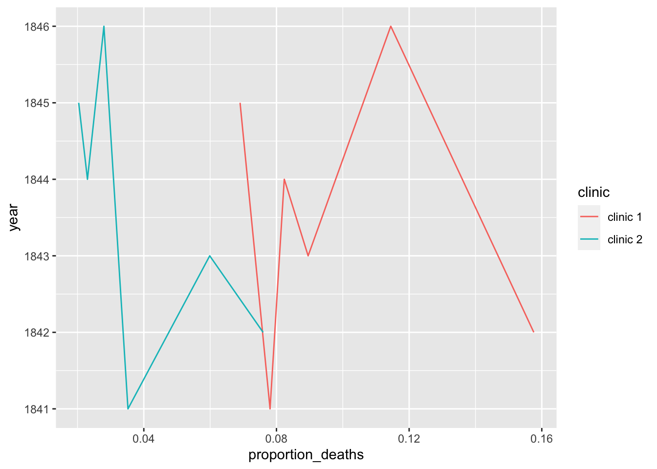
## 6 1846 4010 459 clinic 1 0.114Plot yearly proportion of deaths at the two clinics
ggplot(yearly, aes(x=proportion_deaths, y=year, color=clinic)) +
      geom_line()
Read monthly_deaths.csv into monthly
monthly <- read_csv("monthly_deaths.csv")##
## ── Column specification ────────────────────────────────────────────────────────
## cols(
## date = col_date(format = ""),
## births = col_double(),
## deaths = col_double()
## )Adding a new column with proportion of deaths per no. births
monthly <- monthly %>%
  mutate(proportion_deaths = deaths / births)
head(monthly, 4)
## # A tibble: 4 x 4
## date births deaths proportion_deaths
## <date> <dbl> <dbl> <dbl>
## 1 1841-01-01 254 37 0.146
## 2 1841-02-01 239 18 0.0753
## 3 1841-03-01 277 12 0.0433
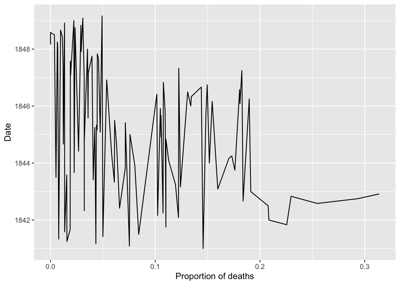
## 4 1841-04-01 255 4 0.0157Plot monthly proportion of deaths
ggplot(monthly, aes(x=proportion_deaths, y=date))+
geom_line() +
labs(x="Proportion of deaths", y="Date")
From this date handwashing was made mandatory
handwashing_start = as.Date('1847-06-01')Add a TRUE/FALSE column to monthly called handwashing_started
monthly <- monthly %>%
  mutate(handwashing_started =
    date >= handwashing_start)
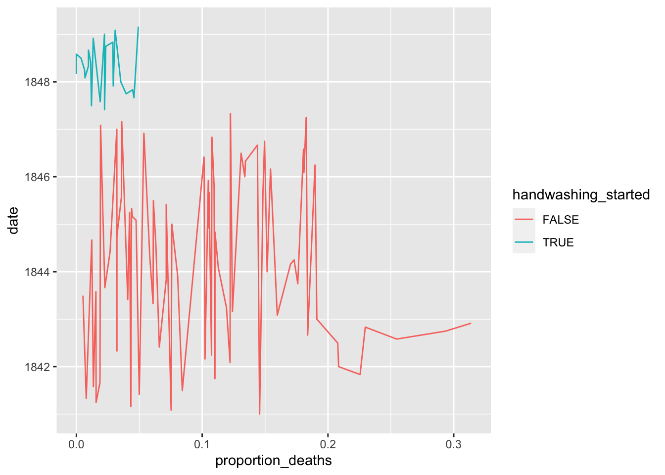
Plot monthly proportion of deaths before and after handwashing
ggplot(monthly, aes(x=proportion_deaths, y=date, color=handwashing_started))+
geom_line()
## Calculating the mean proportion of deaths
## before and after handwashing.
monthly_summary <- monthly %>% group_by(handwashing_started) %>%
summarise(mean(proportion_deaths))
## `summarise()` ungrouping output (override with `.groups` argument)Printing out the summary.
monthly_summary## # A tibble: 2 x 2
## handwashing_started `mean(proportion_deaths)`
## <lgl> <dbl>
## 1 FALSE 0.105
## 2 TRUE 0.0211Calculating a 95% Confidence intrerval using t.test
test_result <- t.test( proportion_deaths ~ handwashing_started, data = monthly)
test_result
##
## Welch Two Sample t-test
##
## data: proportion_deaths by handwashing_started
## t = 9.6101, df = 92.435, p-value = 1.445e-15
## alternative hypothesis: true difference in means is not equal to 0
## 95 percent confidence interval:
## 0.06660662 0.10130659
## sample estimates:
## mean in group FALSE mean in group TRUE
## 0.10504998 0.02109338